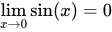
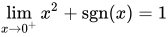
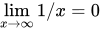
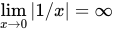
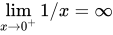
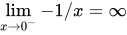
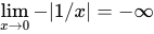
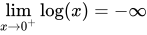
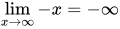
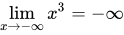
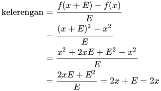
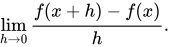
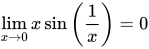
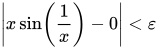
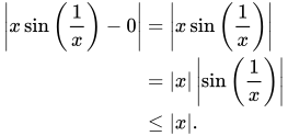
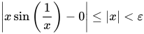
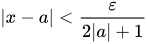
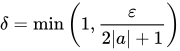
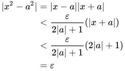
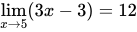
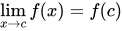
ENSIKLOPEDIA Cari Tekan Enter untuk memulai pencarian cepat. Kembali ke Ensiklopedia Arsip Wikipedia Indonesia Definisi limit (ε, δ) Definisi limit (ε, δ)Definisi matematis limitTemplat:SHORTDESC:Definisi matematis limit Artikel atau sebagian dari artikel ini mungkin diterjemahkan dari (ε, δ)-definition of limit di en.wikipedia.org. Isinya masih belum akurat, karena bagian yang diterjemahkan masih perlu diperhalus dan disempurnakan. Jika Anda menguasai bahasa aslinya, harap pertimbangkan untuk menelusuri referensinya dan menyempurnakan terjemahan ini. Anda juga dapat ikut bergotong royong pada ProyekWiki Perbaikan Terjemahan. (Pesan ini dapat dihapus jika terjemahan dirasa sudah cukup tepat. Lihat pula: panduan penerjemahan artikel) Apabila titik x {\displaystyle x} berada di satuan δ {\displaystyle \delta } dari c {\displaystyle c} , f ( x ) {\displaystyle f(x)} berada di satuan ε {\displaystyle \varepsilon } dari L {\displaystyle L} Dalam kalkulus, definisi limit-(ε, δ) (dibaca "definisi limit epsilon–delta) adalah formalisasi dari pengertian limit. Konsep tersebut karena Augustin-Louis Cauchy, yang tidak pernah memberi nilai definisi limit ( ε , δ {\displaystyle \varepsilon ,\delta } ) dalam Cours d'Analyse, tetapi terkadang digunakan argumen ε , δ {\displaystyle \varepsilon ,\delta } dalam bukti. Ini pertama kali diberikan sebagai definisi formal oleh Bernard Bolzano pada tahun 1817, dan pernyataan modern yang pasti akhirnya diberikan oleh Karl Weierstrass.[1][2] Hal tersebut memberikan ketelitian pada gagasan informal berikut: ungkapan tergantung f ( x ) {\displaystyle f(x)} mendekati nilai L {\displaystyle L} , sebagai variabel x {\displaystyle x} mendekati nilai c {\displaystyle c} jika f ( x ) {\displaystyle f(x)} dapat dibuat sedekat L {\displaystyle L} , dengan mengambil nilai x {\displaystyle x} yang cukup dekat dengan nilai c {\displaystyle c} . Sejarah Meskipun orang Yunani memeriksa proses pembatasan, seperti metode Babilonia, mereka mungkin tidak memiliki konsep yang mirip dengan modern limit.[3] Ketentuan konsep limit muncul pada tahun 1600-an, ketika Pierre de Fermat berusaha menemukan kelerengan dari garis tangen pada suatu titik x {\displaystyle x} dari fungsi seperti f ( x ) = x 2 {\displaystyle f(x)=x^{2}} . Menggunakan kuantitas taknol tetapi hampir nol, E {\displaystyle E} , Fermat melakukan perhitungan berikut: kelerengan = f ( x + E ) − f ( x ) E = ( x + E ) 2 − x 2 E = x 2 + 2 x E + E 2 − x 2 E = 2 x E + E 2 E = 2 x + E = 2 x {\displaystyle {\begin{aligned}{\text{kelerengan}}&={\frac {f(x+E)-f(x)}{E}}\\&={\frac {(x+E)^{2}-x^{2}}{E}}\\&={\frac {x^{2}+2xE+E^{2}-x^{2}}{E}}\\&={\frac {2xE+E^{2}}{E}}=2x+E=2x\end{aligned}}} Kunci dari perhitungan di atas adalah sejak E {\displaystyle E} taknol, salah satunya dapat membagi f ( x + E ) − f ( x ) {\displaystyle f(x+E)-f(x)} dari E {\displaystyle E} , tapi ketika E {\displaystyle E} dekat dengan 0 {\displaystyle 0} , 2 x + E {\displaystyle 2x+E} pada dasarnya adalah 2 x {\displaystyle 2x} .[4] Kuantitas seperti E {\displaystyle E} disebut infinitesimal. Masalah dengan perhitungan ini adalah bahwa para matematikawan zaman itu tidak dapat secara tepat mendefinisikan kuantitas dengan sifat E {\displaystyle E} ,[5] meskipun itu adalah praktik umum untuk 'mengabaikan' infinitesimal pangkat yang lebih tinggi dan ini tampaknya membuahkan hasil yang benar. Masalah ini muncul kembali kemudian pada tahun 1600an di pusat perkembangan kalkulus, karena perhitungan seperti Fermat penting untuk perhitungan turunan. Isaac Newton kalkulus yang dikembangkan pertama kali melalui jumlah yang sangat kecil yang disebut fluks. Dia mengembangkannya dengan mengacu pada gagasan tentang "momen waktu yang sangat kecil..."[6] Namun, Newton kemudian menolak fluks demi teori rasio yang mendekati modern ε – δ {\displaystyle \varepsilon {\text{–}}\delta } definisi limit.[6] Selain itu, Newton menyadari bahwa limit rasio kuantitas lenyap adalah bukan rasio itu sendiri, saat ia menulis: Rasio terakhirnya ... sebenarnya bukan rasio kauntitas terakhirnya, tetapi limit ... yang mana ini dapat didekatkan lebih dekat bahwa perbedaannya lebih kecil dari suatu kuantitas yang diberikan... Sebagai tambahan, Newton terkadang menjelaskan limit dalam istilah yang serupa dengan definisi epsilon–delta.[7] Gottfried Wilhelm Leibniz mengembangkan sebuah infinitesimal oleh dirinya dan mencoba untuk memberikannya dengan sebuah dasar yang setepat-tepatnya, tetapi ini tetap disambut dengan gelisah oleh beberapa matematikawan dan para filsafat.[8] Augustin-Louis Cauchy memberikan sebuah definisi limit dalam hal gagasan lebih primitif yang disebut sebuah kuantitas variabel. Dia tidak pernah memberikan epsilon–delta definisi limit (Grabiner 1981). Beberapa bukti Cauchy berisi indikasi metode epsilon–delta. Whether or not his foundational approach can be considered a harbinger of Weierstrass's is a subject of scholarly dispute. Grabiner feels that it is, while Schubring (2005) disagrees.[diragukan – diskusikan][1] Nakane concludes that Cauchy and Weierstrass gave the same name to different notions of limit.[9] [sumber tepercaya?] Eventually, Weierstrass and Bolzano are credited with providing a rigorous footing for calculus, in the form of the modern ε – δ {\displaystyle \varepsilon {\text{–}}\delta } definition of the limit.[1][10] The need for reference to an infinitesimal E {\displaystyle E} was then removed,[11] and Fermat's computation turned into the computation of the following limit: lim h → 0 f ( x + h ) − f ( x ) h . {\displaystyle \lim _{h\to 0}{\frac {f(x+h)-f(x)}{h}}.} This is not to say that the limiting definition was free of problems as, although it removed the need for infinitesimals, it did require the construction of the real numbers by Richard Dedekind.[12] This is also not to say that infinitesimals have no place in modern mathematics, as later mathematicians were able to rigorously create infinitesimal quantities as part of the hyperreal number or surreal number systems. Moreover, it is possible to rigorously develop calculus with these quantities and they have other mathematical uses.[13] Contoh yang bekerja Contoh 1 Ini akan menunjukkan bahwa lim x → 0 x sin ( 1 x ) = 0 {\displaystyle \lim _{x\to 0}x\sin {\left({\frac {1}{x}}\right)}=0} . Diberikan ε > 0 {\displaystyle \varepsilon >0} , δ > 0 {\displaystyle \delta >0} diperlukan sehingga | x − 0 | < δ {\displaystyle |x-0|<\delta } menyiratkan | x sin ( 1 x ) − 0 | < ε {\displaystyle \left|x\sin \left({\frac {1}{x}}\right)-0\right|<\varepsilon } . Karena sinus dibatasi di atas 1 {\displaystyle 1} dan di bawahnya oleh − 1 {\displaystyle -1} , | x sin ( 1 x ) − 0 | = | x sin ( 1 x ) | = | x | | sin ( 1 x ) | ≤ | x | . {\displaystyle {\begin{aligned}\left|x\sin {\left({\frac {1}{x}}\right)}-0\right|&=\left|x\sin {\left({\frac {1}{x}}\right)}\right|\\&=|x|\left|\sin {\left({\frac {1}{x}}\right)}\right|\\&\leq |x|.\end{aligned}}} Demikianlah, jika δ = ε {\displaystyle \delta =\varepsilon } dipilih, maka | x | = | x − 0 | < δ {\displaystyle |x|=|x-0|<\delta } menyiratkan | x sin ( 1 x ) − 0 | ≤ | x | < ε {\displaystyle \left|x\sin {\left({\frac {1}{x}}\right)}-0\right|\leq |x|<\varepsilon } , yang melengkapi buktinya. Contoh 2 Pernyataan lim x → a x 2 = a 2 {\displaystyle \lim _{x\to a}x^{2}=a^{2}} akan dibuktikan untuk suatu bilangan real a {\displaystyle a} . Diberikan ε > 0 {\displaystyle \varepsilon >0} , δ > 0 {\displaystyle \delta >0} akan ditemukan sehingga | x − a | < δ {\displaystyle |x-a|<\delta } menyiratkan | x 2 − a 2 | < ε {\displaystyle |x^{2}-a^{2}|<\varepsilon } . Dimulai dengan memfaktorkan: | x 2 − a 2 | = | ( x − a ) ( x + a ) | = | x − a | | x + a | {\displaystyle |x^{2}-a^{2}|=|(x-a)(x+a)|=|x-a||x+a|} . Istilah | x − a | {\displaystyle |x-a|} dibatasi oleh δ {\displaystyle \delta } jadi batas dari 1 dapat kita misalkan, dan kemudian sesuatu yang lebih kecil daripadanya dapat diambil untuk δ {\displaystyle \delta } .[14] Jadi, ini dianggap bahwa | x − a | < 1 {\displaystyle |x-a|<1} . Karena | x | − | y | ≤ | x − y | {\displaystyle |x|-|y|\leq |x-y|} berlaku pada umumnya untuk bilangan real x {\displaystyle x} dan y {\displaystyle y} , kita memiliki | x | − | a | ≤ | x − a | < 1 {\displaystyle |x|-|a|\leq |x-a|<1} . Dengan demikian, | x | < 1 + | a | {\displaystyle |x|<1+|a|} . Dengan demikian, melalui pertidaksamaan segitiga, | x + a | ≤ | x | + | a | < 2 | a | + 1. {\displaystyle |x+a|\leq |x|+|a|<2|a|+1.} Dengan demikian, jika kita menganggapnya lebih jauh bahwa | x − a | < ε 2 | a | + 1 {\displaystyle |x-a|<{\frac {\varepsilon }{2|a|+1}}} maka | x 2 − a 2 | < ε {\displaystyle |x^{2}-a^{2}|<\varepsilon } Singkatnya, δ = min ( 1 , ε 2 | a | + 1 ) {\displaystyle \delta =\min {\left(1,{\frac {\varepsilon }{2|a|+1}}\right)}} adalah himpunannya. Jadi, jika | x − a | < δ {\displaystyle |x-a|<\delta } , maka | x 2 − a 2 | = | x − a | | x + a | < ε 2 | a | + 1 ( | x + a | ) < ε 2 | a | + 1 ( 2 | a | + 1 ) = ε {\displaystyle {\begin{aligned}|x^{2}-a^{2}|&=|x-a||x+a|\\&<{\frac {\varepsilon }{2|a|+1}}(|x+a|)\\&<{\frac {\varepsilon }{2|a|+1}}(2|a|+1)\\&=\varepsilon \end{aligned}}} Dengan demikian, kita memiliki sebuah δ {\displaystyle \delta } sehingga | x − a | < δ {\displaystyle |x-a|<\delta } menyiratkan | x 2 − a 2 | < ε {\displaystyle |x^{2}-a^{2}|<\varepsilon } . Dengan demikian, kita telah menunjukkan bahwa lim x → a x 2 = a 2 {\displaystyle \lim _{x\to a}x^{2}=a^{2}} untuk suatu bilangan real a {\displaystyle a} . Contoh 3 Pernyataan lim x → 5 ( 3 x − 3 ) = 12 {\displaystyle \lim _{x\to 5}(3x-3)=12} akan dibuktikan. Ini mudah dibuktikan melalui pemahaman grafis limit, dan demikian berfungsi sebagai dasar-dasar yang kuat untuk induksi pembuktiannya. Menurut definisi formal di atas, sebuah pernyataan limit adalah benar jika dan hanya jika membatasi x {\displaystyle x} ke satuan δ {\displaystyle \delta } dari c {\displaystyle c} akan pasti membatasi f ( x ) {\displaystyle f(x)} ke satuan ε {\displaystyle \varepsilon } dari L {\displaystyle L} . Dalam kasus yang spesifik, ini berarti bahwa pernyataan tersebut benar jika dan hanya jika membatasi x {\displaystyle x} ke satuan δ {\displaystyle \delta } dari 5 akan pasti membatasi 3 x − 3 {\displaystyle 3x-3} ke satuan ε {\displaystyle \varepsilon } dari 12. Kunci secara keseluruhan untuk membuktikan implikasi ini adalah untuk menunjukkan bagaimana δ {\displaystyle \delta } dan ε {\displaystyle \varepsilon } harus berkaitan dengan satu sama lain sehingga implikasinya berlaku. Secara matematis, ini akan menunjukkan bahwa 0 < | x − 5 | < δ ⇒ | ( 3 x − 3 ) − 12 | < ε {\displaystyle 0<|x-5|<\delta \ \Rightarrow \ |(3x-3)-12|<\varepsilon } . Dengan menyederhanakan, memfaktorkan, dan membagi 3 di ruas kanan implikasi menghasilkan | x − 5 | < ε 3 {\displaystyle |x-5|<{\frac {\varepsilon }{3}}} , yang secara langsung memberikan nilai yang diperlukan jika δ = ε / 3 {\displaystyle \delta =\varepsilon /3} dipilih. Dengan demikian, buktinya terselesaikan. Kunci mengenai bukti tersebut terletak dalam kemampuan salah satunya untuk memilih batas-batas di x {\displaystyle x} , dam kemudian menyimpulkan batas-batas berpadanan di f ( x ) {\displaystyle f(x)} , yang mana dalam kasus ini berkaitan dengan sebuah faktor dari 3, yang secara keseluruhan karena kemiringan dari 3 di garis y = 3 x − 3 {\displaystyle y=3x-3} . Kekontinuan Sebuah fungsi f {\displaystyle f} dikatakan kontinu di c {\displaystyle c} jika keduanya didefinisikan di c {\displaystyle c} dan nilainya di c {\displaystyle c} sama dengan limit dari f {\displaystyle f} ketika x {\displaystyle x} mendekati c {\displaystyle c} : lim x → c f ( x ) = f ( c ) {\displaystyle \lim _{x\to c}f(x)=f(c)} . Definisi ( ε , δ ) {\displaystyle (\varepsilon ,\delta )} untuk sebuah fungsi kontinu dapat diperoleh dari definisi limit dengan menggantikan 0 < | x − c | < δ {\displaystyle 0<|x-c|<\delta } dengan | x − c | < δ {\displaystyle |x-c|<\delta } , untuk memastikan bahwa f {\displaystyle f} didefinisikan di c {\displaystyle c} dan sama dengan limitnya. Sebuah fungsi f {\displaystyle f} dikatakan kontinu di selang I {\displaystyle I} jiak fungsi f {\displaystyle f} kontinu di setiap titik c {\displaystyle c} dari I {\displaystyle I} . Perbandingan dengan definisi infinitesimal Keisler proved that a hyperreal definition of limit reduces the logical quantifier complexity by two quantifiers.[15] Namely, f ( x ) {\displaystyle f(x)} converges to a limit L as x {\displaystyle x} tends to a if and only if the value f ( x + e ) {\displaystyle f(x+e)} is infinitely close to L for every infinitesimal e. (See Microcontinuity for a related definition of continuity, essentially due to Cauchy.) Infinitesimal calculus textbooks based on Robinson's approach provide definitions of continuity, derivative, and integral at standard points in terms of infinitesimals. Once notions such as continuity have been thoroughly explained via the approach using microcontinuity, the epsilon–delta approach is presented as well. Karel Hrbáček argues that the definitions of continuity, derivative, and integration in Robinson-style non-standard analysis must be grounded in the ε–δ method, in order to cover also non-standard values of the input.[16] Błaszczyk et al. argue that microcontinuity is useful in developing a transparent definition of uniform continuity, and characterize the criticism by Hrbáček as a "dubious lament".[17] Hrbáček proposes an alternative non-standard analysis, which (unlike Robinson's) has many "levels" of infinitesimals, so that limits at one level can be defined in terms of infinitesimals at the next level.[18] Keluarga definisi limit formal Tidak ada definisi limit yang tunggal - adanya seluruh definisi keluarga. Ini dikarenakan kehadiran takhingga, dan konsep limit "dari sebelah kanan"" dan "dari sebelah kiri". Limit itu sendiri dapat menjadi sebuah nilai terhingga, ∞ {\displaystyle \infty } , atau − ∞ {\displaystyle -\infty } . Nilai yang mendekati oleh x {\displaystyle x} juga dapat menjadi nilai terhingga, ∞ {\displaystyle \infty } , atau − ∞ {\displaystyle -\infty } , dan jika ini merupakan sebuah nilai terhingga, ini dapat mendekati dari kiri atau dari kanan. Biasanya, setiap kombinasinya diberikan definisi itu sendiri, seperti di bawah ini:NotasiDefinisiContoh lim x → c {\displaystyle \lim _{x\to {\color {Green}c}}} f ( x ) = {\displaystyle f(x)=} L {\displaystyle {\color {Red}L}} ⟺ {\displaystyle \iff } ∀ ε > 0 , {\displaystyle {\color {Red}\forall \varepsilon >0,}} ∃ δ > 0 , {\displaystyle {\color {Green}\exists \delta >0,}} ∀ x ∈ D , {\displaystyle \forall x\in D,} c − δ < {\displaystyle {\color {Green}c-\delta }<} x {\displaystyle x} < c + δ {\displaystyle <{\color {Green}c+\delta }} ⇒ {\displaystyle \Rightarrow } L − ε < {\displaystyle {\color {Red}L-\varepsilon }<} f ( x ) {\displaystyle f(x)} < L + ε {\displaystyle <{\color {Red}L+\varepsilon }} lim x → 0 sin ( x ) = 0 {\displaystyle \lim _{x\to 0}\sin(x)=0} lim x → c + {\displaystyle \lim _{x\to {\color {Green}c^{+}}}} f ( x ) = {\displaystyle f(x)=} L {\displaystyle {\color {Red}L}} ⟺ {\displaystyle \iff } ∀ ε > 0 , {\displaystyle {\color {Red}\forall \varepsilon >0,}} ∃ δ > 0 , {\displaystyle {\color {Green}\exists \delta >0,}} ∀ x ∈ D , {\displaystyle \forall x\in D,} c < {\displaystyle {\color {Green}c}<} x {\displaystyle x} < c + δ {\displaystyle <{\color {Green}c+\delta }} ⇒ {\displaystyle \Rightarrow } L − ε < {\displaystyle {\color {Red}L-\varepsilon }<} f ( x ) {\displaystyle f(x)} < L + ε {\displaystyle <{\color {Red}L+\varepsilon }} lim x → 0 + x 2 + sgn ( x ) = 1 {\displaystyle \lim _{x\to 0^{+}}x^{2}+\operatorname {sgn}(x)=1} lim x → c − {\displaystyle \lim _{x\to {\color {Green}c^{-}}}} f ( x ) = {\displaystyle f(x)=} L {\displaystyle {\color {Red}L}} ⟺ {\displaystyle \iff } ∀ ε > 0 , {\displaystyle {\color {Red}\forall \varepsilon >0,}} ∃ δ > 0 , {\displaystyle {\color {Green}\exists \delta >0,}} ∀ x ∈ D , {\displaystyle \forall x\in D,} c − δ < {\displaystyle {\color {Green}c-\delta }<} x {\displaystyle x} < c {\displaystyle <{\color {Green}c}} ⇒ {\displaystyle \Rightarrow } L − ε < {\displaystyle {\color {Red}L-\varepsilon }<} f ( x ) {\displaystyle f(x)} < L + ε {\displaystyle <{\color {Red}L+\varepsilon }} lim x → 0 − x 2 + sgn ( x ) = − 1 {\displaystyle \lim _{x\to 0^{-}}x^{2}+\operatorname {sgn}(x)=-1} lim x → ∞ {\displaystyle \lim _{x\to {\color {Green}\infty }}} f ( x ) = {\displaystyle f(x)=} L {\displaystyle {\color {Red}L}} ⟺ {\displaystyle \iff } ∀ ε > 0 , {\displaystyle {\color {Red}\forall \varepsilon >0,}} ∃ M > 0 , {\displaystyle {\color {Green}\exists M>0,}} ∀ x ∈ D , {\displaystyle \forall x\in D,} M < {\displaystyle {\color {Green}M}<} x {\displaystyle x} ⇒ {\displaystyle \Rightarrow } L − ε < {\displaystyle {\color {Red}L-\varepsilon }<} f ( x ) {\displaystyle f(x)} < L + ε {\displaystyle <{\color {Red}L+\varepsilon }} lim x → ∞ 1 / x = 0 {\displaystyle \lim _{x\to \infty }1/x=0} lim x → − ∞ {\displaystyle \lim _{x\to {\color {Green}-\infty }}} f ( x ) = {\displaystyle f(x)=} L {\displaystyle {\color {Red}L}} ⟺ {\displaystyle \iff } ∀ ε > 0 , {\displaystyle {\color {Red}\forall \varepsilon >0,}} ∃ M < 0 , {\displaystyle {\color {Green}\exists M<0,}} ∀ x ∈ D , {\displaystyle \forall x\in D,} x {\displaystyle x} < M {\displaystyle <{\color {Green}M}} ⇒ {\displaystyle \Rightarrow } L − ε < {\displaystyle {\color {Red}L-\varepsilon }<} f ( x ) {\displaystyle f(x)} < L + ε {\displaystyle <{\color {Red}L+\varepsilon }} lim x → − ∞ e x = 0 {\displaystyle \lim _{x\to -\infty }e^{x}=0} lim x → c {\displaystyle \lim _{x\to {\color {Green}c}}} f ( x ) = {\displaystyle f(x)=} ∞ {\displaystyle {\color {Red}\infty }} ⟺ {\displaystyle \iff } ∀ N > 0 , {\displaystyle {\color {Red}\forall N>0,}} ∃ δ > 0 , {\displaystyle {\color {Green}\exists \delta >0,}} ∀ x ∈ D , {\displaystyle \forall x\in D,} c − δ < {\displaystyle {\color {Green}c-\delta }<} x {\displaystyle x} < c + δ {\displaystyle <{\color {Green}c+\delta }} ⇒ {\displaystyle \Rightarrow } N < {\displaystyle {\color {Red}N}<} f ( x ) {\displaystyle f(x)} lim x → 0 | 1 / x | = ∞ {\displaystyle \lim _{x\to 0}|1/x|=\infty } lim x → c + {\displaystyle \lim _{x\to {\color {Green}c^{+}}}} f ( x ) = {\displaystyle f(x)=} ∞ {\displaystyle {\color {Red}\infty }} ⟺ {\displaystyle \iff } ∀ N > 0 , {\displaystyle {\color {Red}\forall N>0,}} ∃ δ > 0 , {\displaystyle {\color {Green}\exists \delta >0,}} ∀ x ∈ D , {\displaystyle \forall x\in D,} c < {\displaystyle {\color {Green}c}<} x {\displaystyle x} < c + δ {\displaystyle <{\color {Green}c+\delta }} ⇒ {\displaystyle \Rightarrow } N < {\displaystyle {\color {Red}N}<} f ( x ) {\displaystyle f(x)} lim x → 0 + 1 / x = ∞ {\displaystyle \lim _{x\to 0^{+}}1/x=\infty } lim x → c − {\displaystyle \lim _{x\to {\color {Green}c^{-}}}} f ( x ) = {\displaystyle f(x)=} ∞ {\displaystyle {\color {Red}\infty }} ⟺ {\displaystyle \iff } ∀ N > 0 , {\displaystyle {\color {Red}\forall N>0,}} ∃ δ > 0 , {\displaystyle {\color {Green}\exists \delta >0,}} ∀ x ∈ D , {\displaystyle \forall x\in D,} c − δ < {\displaystyle {\color {Green}c-\delta }<} x {\displaystyle x} < c {\displaystyle <{\color {Green}c}} ⇒ {\displaystyle \Rightarrow } N < {\displaystyle {\color {Red}N}<} f ( x ) {\displaystyle f(x)} lim x → 0 − − 1 / x = ∞ {\displaystyle \lim _{x\to 0^{-}}-1/x=\infty } lim x → ∞ {\displaystyle \lim _{x\to {\color {Green}\infty }}} f ( x ) = {\displaystyle f(x)=} ∞ {\displaystyle {\color {Red}\infty }} ⟺ {\displaystyle \iff } ∀ N > 0 , {\displaystyle {\color {Red}\forall N>0,}} ∃ M > 0 , {\displaystyle {\color {Green}\exists M>0,}} ∀ x ∈ D , {\displaystyle \forall x\in D,} M < {\displaystyle {\color {Green}M}<} x {\displaystyle x} ⇒ {\displaystyle \Rightarrow } N < {\displaystyle {\color {Red}N}<} f ( x ) {\displaystyle f(x)} lim x → ∞ e x = ∞ {\displaystyle \lim _{x\to \infty }e^{x}=\infty } lim x → − ∞ {\displaystyle \lim _{x\to {\color {Green}-\infty }}} f ( x ) = {\displaystyle f(x)=} ∞ {\displaystyle {\color {Red}\infty }} ⟺ {\displaystyle \iff } ∀ N > 0 , {\displaystyle {\color {Red}\forall N>0,}} ∃ M < 0 , {\displaystyle {\color {Green}\exists M<0,}} ∀ x ∈ D , {\displaystyle \forall x\in D,} x {\displaystyle x} < M {\displaystyle <{\color {Green}M}} ⇒ {\displaystyle \Rightarrow } N < {\displaystyle {\color {Red}N}<} f ( x ) {\displaystyle f(x)} lim x → − ∞ x 2 = ∞ {\displaystyle \lim _{x\to -\infty }x^{2}=\infty } lim x → c {\displaystyle \lim _{x\to {\color {Green}c}}} f ( x ) = {\displaystyle f(x)=} − ∞ {\displaystyle {\color {Red}-\infty }} ⟺ {\displaystyle \iff } ∀ N < 0 , {\displaystyle {\color {Red}\forall N<0,}} ∃ δ > 0 , {\displaystyle {\color {Green}\exists \delta >0,}} ∀ x ∈ D , {\displaystyle \forall x\in D,} c − δ < {\displaystyle {\color {Green}c-\delta }<} x {\displaystyle x} < c + δ {\displaystyle <{\color {Green}c+\delta }} ⇒ {\displaystyle \Rightarrow } f ( x ) {\displaystyle f(x)} < N {\displaystyle <{\color {Red}N}} lim x → 0 − | 1 / x | = − ∞ {\displaystyle \lim _{x\to 0}-|1/x|=-\infty } lim x → c + {\displaystyle \lim _{x\to {\color {Green}c^{+}}}} f ( x ) = {\displaystyle f(x)=} − ∞ {\displaystyle {\color {Red}-\infty }} ⟺ {\displaystyle \iff } ∀ N < 0 , {\displaystyle {\color {Red}\forall N<0,}} ∃ δ > 0 , {\displaystyle {\color {Green}\exists \delta >0,}} ∀ x ∈ D , {\displaystyle \forall x\in D,} c < {\displaystyle {\color {Green}c}<} x {\displaystyle x} < c + δ {\displaystyle <{\color {Green}c+\delta }} ⇒ {\displaystyle \Rightarrow } f ( x ) {\displaystyle f(x)} < N {\displaystyle <{\color {Red}N}} lim x → 0 + log ( x ) = − ∞ {\displaystyle \lim _{x\to 0^{+}}\log(x)=-\infty } lim x → c − {\displaystyle \lim _{x\to {\color {Green}c^{-}}}} f ( x ) = {\displaystyle f(x)=} − ∞ {\displaystyle {\color {Red}-\infty }} ⟺ {\displaystyle \iff } ∀ N < 0 , {\displaystyle {\color {Red}\forall N<0,}} ∃ δ > 0 , {\displaystyle {\color {Green}\exists \delta >0,}} ∀ x ∈ D , {\displaystyle \forall x\in D,} c − δ < {\displaystyle {\color {Green}c-\delta }<} x {\displaystyle x} < c {\displaystyle <{\color {Green}c}} ⇒ {\displaystyle \Rightarrow } f ( x ) {\displaystyle f(x)} < N {\displaystyle <{\color {Red}N}} lim x → 0 − 1 / x = − ∞ {\displaystyle \lim _{x\to 0^{-}}1/x=-\infty } lim x → ∞ {\displaystyle \lim _{x\to {\color {Green}\infty }}} f ( x ) = {\displaystyle f(x)=} − ∞ {\displaystyle {\color {Red}-\infty }} ⟺ {\displaystyle \iff } ∀ N < 0 , {\displaystyle {\color {Red}\forall N<0,}} ∃ M > 0 , {\displaystyle {\color {Green}\exists M>0,}} ∀ x ∈ D , {\displaystyle \forall x\in D,} M < {\displaystyle {\color {Green}M}<} x {\displaystyle x} ⇒ {\displaystyle \Rightarrow } f ( x ) {\displaystyle f(x)} < N {\displaystyle <{\color {Red}N}} lim x → ∞ − x = − ∞ {\displaystyle \lim _{x\to \infty }-x=-\infty } lim x → − ∞ {\displaystyle \lim _{x\to {\color {Green}-\infty }}} f ( x ) = {\displaystyle f(x)=} − ∞ {\displaystyle {\color {Red}-\infty }} ⟺ {\displaystyle \iff } ∀ N < 0 , {\displaystyle {\color {Red}\forall N<0,}} ∃ M < 0 , {\displaystyle {\color {Green}\exists M<0,}} ∀ x ∈ D , {\displaystyle \forall x\in D,} x {\displaystyle x} < M {\displaystyle <{\color {Green}M}} ⇒ {\displaystyle \Rightarrow } f ( x ) {\displaystyle f(x)} < N {\displaystyle <{\color {Red}N}} lim x → − ∞ x 3 = − ∞ {\displaystyle \lim _{x\to -\infty }x^{3}=-\infty } Lihat pula Fungsi kontinu Limit barisan Daftar topik kalkulus Teorema apit Referensi 1 2 3 Grabiner, Judith V. (Maret 1983), "Siapa yang Memberi Anda Epsilon? Cauchy dan Origins of Rigorous Calculus" (PDF), The American Mathematical Monthly, 90 (3): 185–194, doi:10.2307/2975545, JSTOR 2975545, diarsipkan (PDF) dari versi aslinya tanggal 2009-05-04, diakses tanggal 2009-05-01 ↑ Cauchy, A.-L. (1823), "Septième Leçon – Valeurs de quelques expressions qui se présentent sous les formes indéterminées ∞ ∞ , ∞ 0 , … {\displaystyle {\frac {\infty }{\infty }},\infty ^{0},\ldots } Relation qui existe entre le rapport aux différences finies et la fonction dérivée", Résumé des leçons données à l'école royale polytechnique sur le calcul infinitésimal, Paris, diarsipkan dari asli tanggal 2009-05-04, diakses tanggal 2009-05-01, p. 44. Pemeliharaan CS1: Postscript (link). Accessed 2009-05-01. ↑ Stillwell, John (1989). Matematika dan Sejarahnya. New York: Springer-Verlag. hlm. 38–39. ISBN 978-1-4899-0007-4. ↑ Stillwell, John (1989). Matematika dan Sejarahnya. New York: Springer-Verlag. hlm. 104. ISBN 978-1-4899-0007-4. ↑ Stillwell, John (1989). Matematika dan Sejarahnya. New York: Springer-Verlag. hlm. 106. ISBN 978-1-4899-0007-4. 1 2 Buckley, Benjamin Lee (2012). Perdebatan kontinuitas: Dedekind, Cantor, du Bois-Reymond dan Peirce tentang kontinuitas dan infinitesimal. hlm. 31. ISBN 9780983700487. ↑ Pourciau, B. (2001), "Newton and the Notion of Limit", Historia Mathematica, 28 (1): 18–30, doi:10.1006/hmat.2000.2301 ↑ Buckley, Benjamin Lee (2012). The continuity debate : Dedekind, Cantor, du Bois-Reymond and Peirce on continuity and infinitesimals. hlm. 32. ISBN 9780983700487. ↑ Nakane, Michiyo. Did Weierstrass's differential calculus have a limit-avoiding character? His definition of a limit in ε−δ style. BSHM Bull. 29 (2014), no. 1, 51–59. ↑ Cauchy, A.-L. (1823), "Septième Leçon - Valeurs de quelques expressions qui se présentent sous les formes indéterminées ∞ ∞ , ∞ 0 , … {\displaystyle {\frac {\infty }{\infty }},\infty ^{0},\ldots } Relation qui existe entre le rapport aux différences finies et la fonction dérivée", Résumé des leçons données à l'école royale polytechnique sur le calcul infinitésimal, Paris, diarsipkan dari asli tanggal 2009-05-04, diakses tanggal 2009-05-01, p. 44. Pemeliharaan CS1: Postscript (link). ↑ Buckley, Benjamin Lee (2012). The continuity debate : Dedekind, Cantor, du Bois-Reymond and Peirce on continuity and infinitesimals. hlm. 33. ISBN 9780983700487. ↑ Buckley, Benjamin Lee (2012). The continuity debate : Dedekind, Cantor, du Bois-Reymond and Peirce on continuity and infinitesimals. hlm. 32–35. ISBN 9780983700487. ↑ Tao, Terence (2008). Structure and randomness : pages from year one of a mathematical blog. Providence, R.I.: American Mathematical Society. hlm. 95–110. ISBN 978-0-8218-4695-7. ↑ Spivak, Michael (2008). Kalkulus (Edisi 4th). Houston, Tex.: Publish or Perish. hlm. 95. ISBN 978-0914098911. ↑ Keisler, H. Jerome (2008), "Quantifiers in limits" (PDF), Andrzej Mostowski and foundational studies, IOS, Amsterdam, hlm. 151–170 ↑ Hrbacek, K. (2007), "Stratified Analysis?", dalam Van Den Berg, I.; Neves, V. (ed.), The Strength of Nonstandard Analysis, Springer ↑ Błaszczyk, Piotr; Katz, Mikhail; Sherry, David (2012), "Ten misconceptions from the history of analysis and their debunking", Foundations of Science, 18: 43–74, arXiv:1202.4153, Bibcode:2012arXiv1202.4153B, doi:10.1007/s10699-012-9285-8, S2CID 119134151 ↑ Hrbacek, K. (2009). "Relative set theory: Internal view". Journal of Logic and Analysis. 1. Basis data pengawasan otoritas: Nasional Jepang